About Limit Analysis

Limit analysis is one of the analytical methods permitted in the nuclear code RCC-MR.

Compared to conventional methods that linearise stress (by drawing evaluation lines) and evaluate it, this method offers the advantage of more easily evaluating plastic collapse. In linearisation evaluation, there is a challenge that the evaluation lines are not always explicitly defined, nor is the criterion for judging whether the calculated stress is peak stress or local stress, and the evaluation method can vary slightly depending on the analyst.

Limit analysis has been used in the structural analysis of ITER's vacuum vessel, and is a method employed particularly for evaluating areas prone to stress concentration, such as near the base of ports.

In elastic analysis, once the generated stress exceeds the yield stress, the strain amount cannot be appropriately evaluated thereafter, making it impossible to evaluate the collapse load itself. On the other hand, while elasto-plastic analysis (analysis that considers material non-linearity) allows for evaluation closer to actual behaviour, it presents challenges such as setting up preconditions for handling non-linearity and increased computational cost. Limit analysis is an analytical method positioned between these two, and by combining the two concepts of the lower bound theorem and a perfectly plastic body, it is possible to evaluate the collapse load on the safe side through static structural analysis.

Lower Bound Theorem

This is a theorem stating that if a stress distribution can be found that is in equilibrium and does not exceed the yield stress anywhere, then the load is guaranteed to be less than or equal to the true collapse load. This theorem mathematically guarantees that an evaluation on the safe side is achieved, even if the analyst does not strictly satisfy the compatibility conditions of deformation when determining the stress distribution, as long as equilibrium and yield conditions are met.

Perfectly Plastic Body

This refers to a model that approximates the stress-strain diagram with two straight lines (bilinear). It is a simplified model where stress and strain increase proportionally and monotonically until the yield stress is reached, after which strain increases while stress remains constant.

Actual Judgement Method

There are broadly two approaches to the practical determination of collapse load. One is the "twice elastic gradient method", where the load is increased while plotting the displacement (or angle of rotation) at a representative point, and the intersection of the collapse load with a straight line that is half the gradient in the elastic region is considered the collapse load. The other is a method where the load at the point when local strain reaches a certain reference value (which varies depending on the object and applicable standards) is considered the collapse load. In either method, by comparing the calculated collapse load with the actual design load, the design margin can be calculated.

Verification with ANSYS: Collapse Load Evaluation in a Cantilever Beam Model

To deepen the understanding of the theory, a numerical analysis was performed using ANSYS with a simple cantilever beam model, and its consistency with the theoretical value was confirmed.

Model Conditions

• Cross-section: 10 mm × 10 mm (rectangular cross-section)
• Length: 100 mm
• Material Model: Perfectly plastic body (bilinear model with yield stress of 200 MPa and zero hardening coefficient)
• Boundary Conditions: Root completely fixed (Fixed Support), concentrated load gradually applied at the tip

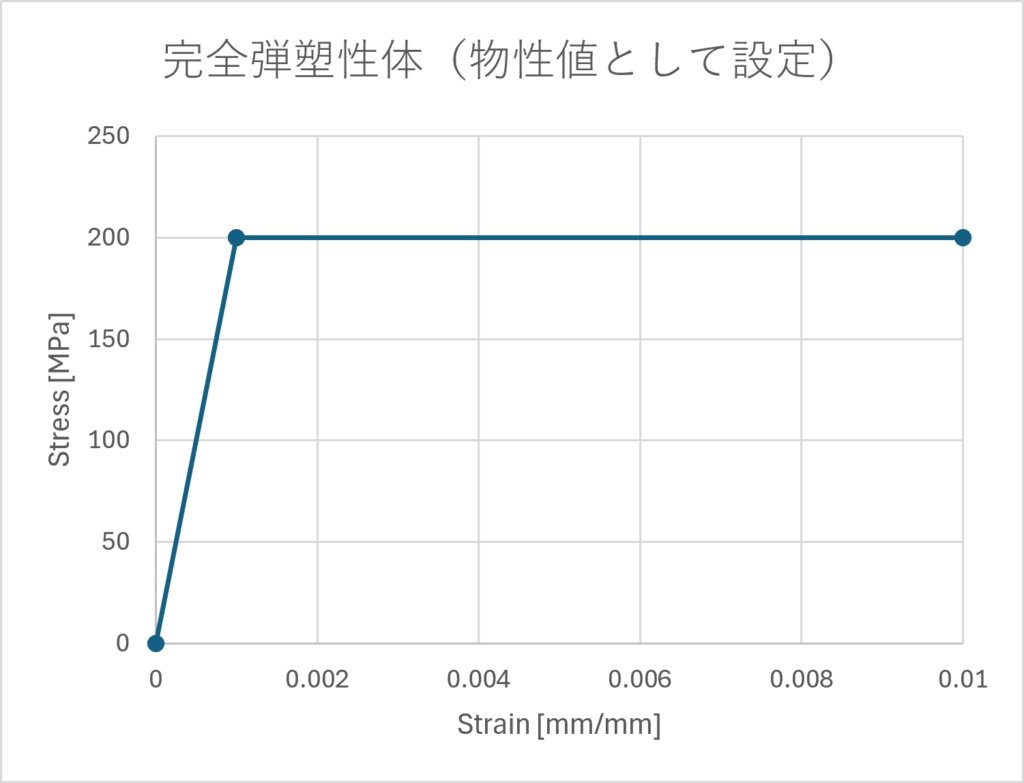
[Figure 1: Material Model (Stress-Strain Diagram)]

As for the material properties, a perfectly plastic body was set up, which behaves elastically until the yield stress of 200 MPa is reached, and after yielding, the strain increases while the stress remains constant. It can be confirmed that it is input as a bilinear model, which is a two-straight-line model as per the theory.

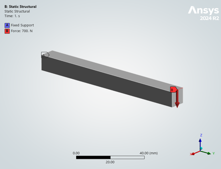
[Figure 2: Boundary Conditions]

Comparison with Theoretical Value

The plastic moment Mp for a rectangular cross-section cantilever beam is given by

   

Substituting the conditions for this case ( σy = 200 MPa, b = h = 10 mm ), we get

   

From the relationship between the tip load P and the root moment Mp (Mp = P・L), the theoretical collapse load is calculated as

   

which is obtained.

Analysis Results: Load-Strain Curve and Twice Elastic Gradient Method

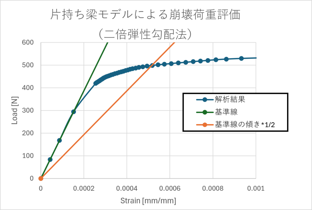
[Figure 3: Collapse Load Evaluation Graph (Twice Elastic Gradient Method)]

The load-strain curve obtained while gradually increasing the tip load is shown in the figure above. By drawing a straight line with half the gradient of the elastic region (reference line) and reading the intersection point with the load-strain curve, the collapse load is approximately 500 N, which is almost perfectly consistent with the theoretical value (500 N).

In the load-displacement curve using tip displacement, the influence of local yielding is relatively small compared to the deformation of the entire beam, so nonlinearities are less likely to appear as clearly as when viewed by strain. The reason for using strain to determine the collapse load in this case is to more directly capture the behaviour at the fixed end where the plastic hinge forms.

Verification by Stress and Strain Distribution

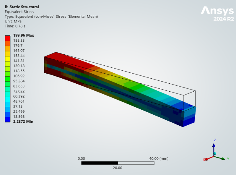
[Figure 4: Stress Contour (Elemental Mean Display)]

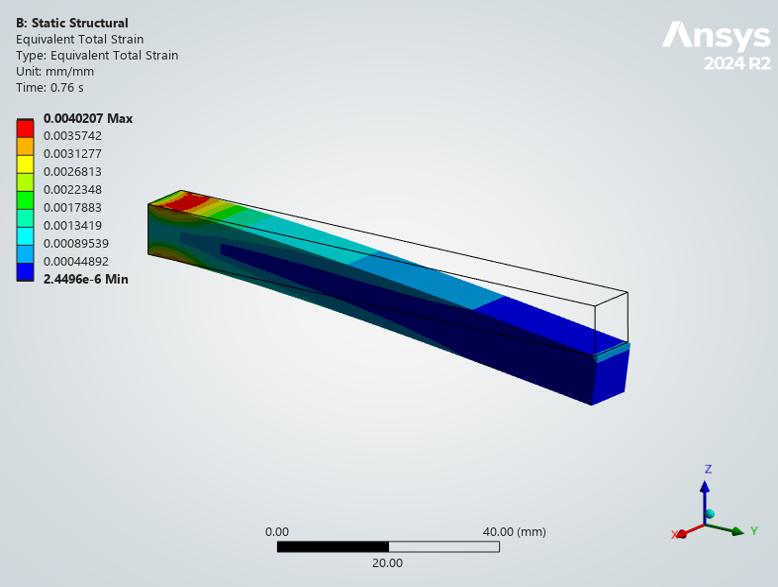
[Figure 5: Strain Contour]

Checking the stress distribution under load conditions exceeding the collapse load (700 N), the maximum stress near the root is 199.96 MPa, confirming that it does not exceed the set yield stress of 200 MPa. Concurrently, checking the strain distribution under the same conditions reveals that significant plastic strain (maximum approximately 0.004 mm/mm) occurs near the root where the stress has reached the yield stress. The fact that both stress and strain distributions correspond near the root supports that this behaviour is a result of plasticisation actually progressing, rather than numerical error.

Note that depending on how the stress contour is displayed (nodal average or elemental average), values that apparently slightly exceed the yield stress may be displayed due to extrapolation and averaging between adjacent elements. In this case, by using the Elemental Mean display, we have confirmed results consistent with theory, which do not exceed the yield stress set in the material model.

Summary

Although it is a simple cantilever beam model, we have confirmed that the results of theoretical calculations (collapse load from fully plastic moment) and numerical analysis by ANSYS (determination by the twice-elastic-gradient method) are almost perfectly consistent. In addition, from both stress and strain contour diagrams, we were able to visually confirm that plasticisation is actually progressing in the region exceeding the collapse load.